A Brief History of PCA
The First Application of PCA: The Solar System
The first known scientific application of Principal Components Analysis (PCA) can fairly be said to have been carried off by the Medieval astronomers, such as Kepler and Galileo. Of course, it wasn't called by that name back then. It was used almost unconsicously, as brilliant men struggled to comprehend the complex motions of the planets.
The Medieval astronomers used the technique to simplify the motion of the Solar System, which resulted in a stunning insight into the Laws of motion of Heavenly Bodies (free-floating objects in space under gravitational forces). This in turn led to Newton's Laws of Physics, and started up the modern scientific era. (Quite a feat for one small technique!)
So its easy to see how PCA got its reputation as the 'Queen' of the Multivariate Analysis Methods.
Linear Transforms
What the early astronomers did is what is known today as a simple Linear Transformation of coordinates. Almost every high school graduate will have at least had a taste of them. Its more than simply switching viewpoints. Obviously we can't land on the Sun, and watch everything from there.
Instead, we have to convert all the measurements we have taken from Earth, to new measurements that would have been recorded, had we done them from the Sun. There are two steps to this. First we have to figure out how the Sun is moving relative to the Earth. Then we compensate for this motion by adjusting every one of our measurements.
To make this tedious and complicated task easy, we use Matrix Algebra or Linear Algebra techniques. We take related groups of our measurements for each 'point' (for instance an X, Y, or Z coordinate at some time T), and multiply the whole thing by a 'matrix' (a box of numbers or functions) according to a special set of rules. This gives us a new set of measurements (X2, Y2, Z2, T2) which we plot on a new 'map' or graph of planet motion.
The result is dramatic: We go from a map of motion for the planets like this (how it looks from Earth):
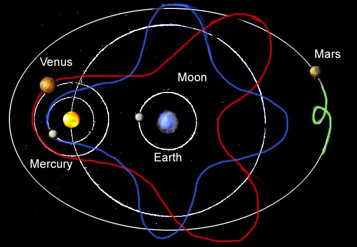
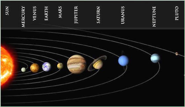
To a map of the Solar System like this (how it looks from the Sun):
Why did it Work?
The increase in order and clarity is shocking. But it is not simple elegance that makes the new presentation profound. This would be to completely misunderstand our result. What makes the new version powerful is its explanatory and predictive power.
The model with the Sun in the center strongly suggests the Sun itself is the organizing force in the Solar System. And indeed this insight led Newton to a gravity theory which was able to account for the planetary orbits, and all generally observed motion.
But it would be absurd to say that all this came about from a simple substitution of reference frame, or transposition of coordinates. How did the astronomers know which part of the Solar System to use as a 'fixed point'? This was hardly obvious.
And more to the point, no 'automated' Principal Components Analysis trick performed on the raw data from earthly observations could have pulled this rabbit out of the hat. We'll see why in a minute. It happened in stages through a series of observations, struggles and insights.
Absolute Motion: Unprovable
Most people will have been told in school that Galileo "proved" that the Earth circles the Sun, and that the nasty and bigoted Church authorities and their egotistical "Earth-centered" viewpoint were eliminated.
But the historical and scientific facts are quite different. From the moment that Newton proposed the idea of a unique framework of Absolute Rest and the concept of Absolute Motion, other scientists protested strongly.
If all motion must be and can only be detected by comparison to other nearby objects, how can there be such a thing as Absolute motion? All motion must be relative, and simply based upon our viewpoint. It doesn't matter what state of 'motion' we call 'standing still'. All other motions will be based from that, and the same physical 'laws' should apply, whatever viewpoint we are measuring from.
In fact, the rejection of these ideas is what led Mach, and his brilliant student Albert Einstein to attempt to universalize the laws of physics so that all states of motion were equal, and relative (hence the name of Einstein's theory, "Relativity").
So it wasn't 'crazy' to challenge the idea that the Sun was the center of the Universe. According to the logic of the best scientific minds for 300 years, all motion should be 'relative'. Copernicus and Galileo were no more right than the stuffy Church leaders, and had by no means proved any such thesis.
The best that could be said was, placing the Sun at the center of the Solar System (not the universe!) greatly simplified the picture, and assisted in our understanding of gravitational forces, and was in the end extremely practical for many kinds of calculations. Of course this was a heck of an argument in itself for putting the Sun at the center, and treating it as stationary for most purposes.
No Such Thing as Orbits
As it turns out, although making the Sun the center of the Solar System is a neat trick, placing all the planets into tidy near-circular orbits, even this is really a bit of a fraud, when the big picture is taken into consideration. This tidy picture quickly dissolves again when we consider the motion of the Solar System itself, as it travels along in a spiral arm of the galaxy we live in, called the Milky Way.
Let's see how it suddenly gets complicated all over again.
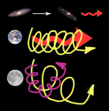
Our galaxy is flying along, apparently away from other nearby galaxies. The Solar System is circling around in our galaxy in one of the spiral arms, cutting a kind of spiral or helix path through space. The Earth, circling the Sun, is dragged this way and that as the Sun (center of our Solar System) swings back and forth. The Moon, swinging about the Earth, follows a path that is really a combination of all of these motions, a kind of crazy slinky journey.
The whole Solar System, although making a fairly predictable and even beautiful pattern as it cuts through space, is hardly the simple 'orbit map' it appears from the Sun's viewpoint.

The Moral of the Story
This brief look at PCA techniques in early astronomy shows us a few important lessons.
(1) Principle Component Analysis (PCA) is not new.
The basic ideas and techniques have been around almost as long as Cartesian coordinates, and the connection of algebra to geometry.
(2) PCA is not an 'automatic' process.
In any important analysis of data, a lot of theoretical groundwork, experiment, trial-and-error, and re-thinking of the problem in its details and its larger context is necessary. Theoretical frameworks and hypotheses must be used to make any sense or practical use of the data.
(3) PCA doesn't give the 'right' answer.
Data often contains many spurious patterns, and can have complex layers of independant cause and effect. There is no guarantee that PCA or any other technique will expose the 'correct' pattern in the data, among many. At best, a successful application of PCA will expose the 'loudest' patterns, or the crudest. But only an intelligent theoretical framework can assign importance, relative weights, or even meaning to 'patterns' in data.
The recent history of PCA methods
Karl Pearson developed the mathematical foundation of PCA in 1901 1. Since that time, it has been expanded and honed into a large group of related statistical methods and techniques, and it has been a component in many modern scientific papers.
Many computer software companies and suppliers of technical tools have incorporated PCA into both general purpose and specialized statistical 'packages', so that researchers no longer need to 'reinvent the wheel'. In fact, researchers don't even need to understand the mechanical internal workings of PCA itself, to benefit from its application in many situations.
Its application has flourished in the social sciences, where it was used to quantify and identify phenomena that could not be measured directly, such as ‘health-related quality of life’ 2 or ‘sources of stress’ 3 .
PCA allows the identification of groups of variables that are interrelated via phenomena that cannot be directly observed. This is accomplished by assuming that any observed (manifest) variables are correlated with a small number of underlying phenomena, which cannot be measured directly (latent variables).
Thus, if variable A is related to B, B is related to C and A is related to C it may well be that A, B and C have something in common. In statistical terms, the observed correlation matrix is used to make inferences about the identities of any latent variables. (These would be hidden factors, causes, effects, which in turn might suggest 'laws' or principles directing the process under investigation).
Therefore, PCA is merely an automated and systematic examination of correlations among known variables, aimed at identifying underlying latent principal components (hidden variables of cause or effect). Data can be analyzed by hand without resorting to fancy statistical modeling. However, for large tables of data, the task can be daunting without the aid of techniques like PCA.
(paraphrased from Igor Burstyn, Principal Component Analysis is a Powerful Instrument in Occupational Hygiene Inquiries, Annals of Occupational Hygiene 2004 48(8):655-661)
references:
1. Pearson K. (1901) On lines and planes of closest fit to systems of points in space. Phil Mag; 2: 559–72.
2. Clark JA, Wray N, Brody B et al. (1997) Dimensions of quality of life expressed by men treated for metastatic prostate cancer. Soc Sci Med; 45: 1299–309.
3. Beaton R, Murphy S, Johnson C et al. (1998) Exposure to duty-related incident stressors in urban firefighters and paramedics. J Trauma Stress; 11: 821–8.
Multivariate Data Analysis:
The Big Picture
Multivariate Data Analysis (MDA) is about separating the signal from the noise in sets of data involving many variables, and presenting the results as easy to interpret plots or graphs. Any large complex table of data can in theory be easily transformed into intuitive pictures, summarizing the essential information.
In the field of MDA, several popular methods that are based on mathematical projection have been developed to meet different needs: PCA, PLS, and PLS-DA.
Getting an Overview with PCA
Principal Components Analysis provides a concise overview of a dataset and is often the first step in any analysis. It can be useful for recognising patterns in data: outliers, trends, groups etc.
PCA is a very useful method to analyze numerical data already organized in a two-dimensional table (of M 'observations' by N 'variables'). It allows us to continue analyzing the data ands:
- Quickly identify correlations between the N variables,
- Display the groupings of the M observations (initially described by the N variables) on a low dimensional map, which in turn help identify a variability criterion,
- Build a set of P uncorrelated factors (P <= N ) that can be reused as input for other statistical methods (such as regression).
The limits of PCA stem from the fact that it is a projection method, and sometimes the visualization can lead to false interpretations. There are however some tricks to avoid these pitfalls.
Establishing Relationships with PLS
With Projections to Latent Structures, the aim is to establish relationships between input and output variables, creating predictive models that can be tested by further data collection.
Classification of New Objects with PLS-DA
PLS-Discriminant Analysis is a powerful method for classification. Again, the aim is to create a predictive model, but one which is general and robust enough to accurately classify future unknown samples or measurements.
Summary
Each of these methods or techniques have a variety of related goals associated with them, and their appropriateness and success is partly determined by nature of the problem and the data to which they are applied. They are simply some of the many mathematical tools available to scientific researchers.
Secondly, each method requires that a meaningful framework for the experiment be prepared beforehand, and that the data be properly prepared. Finally, interpretation of the results must be guided by a rational theoretical model with plausible explanatory power, relating the numerical and graphical objects to the real world in an unambiguous and scientific manner.
The Mechanics of PCA
A 'Walk Through'
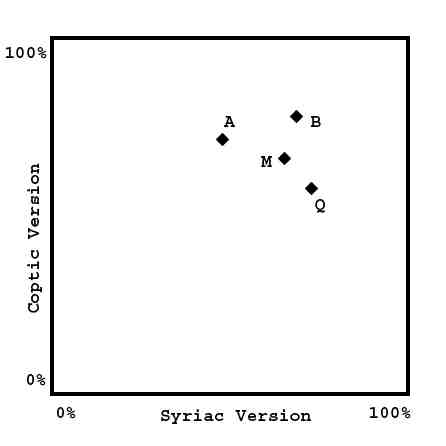
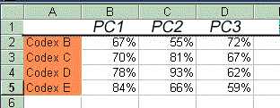
Suppose we are investigating textual patterns in different manuscripts (abbrev. = 'MSS', singular = 'MS'). The numbers in our data-table could refer to the percentage agreement between manuscripts and known Versions (standard translations) or Text-types (what a layman would call a 'version' of a text, i.e., a certain group of associated 'readings'.).
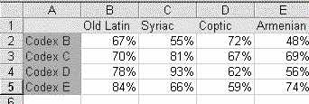
Its hard to see and understand the relationships among and between the MSS and the versions by just staring at numbers. We can't fully interpret most tables by inspection. We need a pictorial representation of the data, a graph or chart.
Converting Numbers into Pictures
By using Multivariate Projection Methods, we can transform the numbers into pictures. Note the names of the columns and rows in our sample data-table. These are the conceptual 'objects' we want to understand (manuscripts and versions).
The first plot is like a map, showing how the MSS relate to each other based on their "agreement profiles" (nearness = agreement). MSS with similar profiles lie close to each other in the map while MSS with different profiles are farther apart. 'Distance' is related to similarity, or affinity. We call such a map a Score Plot. We will see how a plot is created shortly.
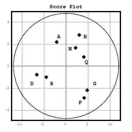
For example, the Alexandrian MSS might cluster together in the top right quadrant while the Byzantine MSS form a cluster to the left.
The co-ordinates of the map (or number scales) are called the first two Principal Components, and the (x,y) values for each object are calculated from all of the data taken together (we'll see how shortly).
Having examined the score plot, it is natural to ask why, say, the Egyptian and Caesarian MSS cluster together. This information can be revealed by the second plot called a Loading Plot.
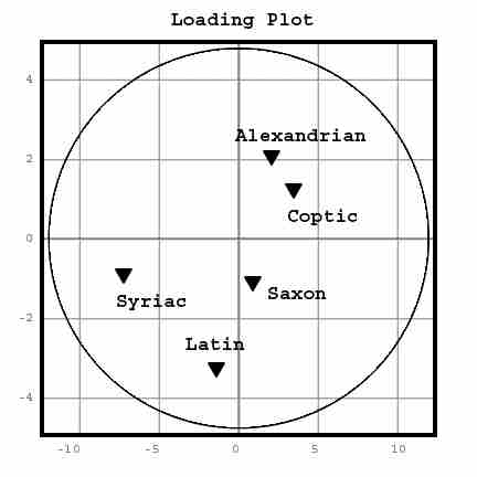
In the top right quadrant (the same area as the Egyptian cluster) we might find Coptic and Alexandrian Versions all of which have close affinities to an Egyptian/Alexandrian Text-type. By contrast, the Byzantine MSS contain many Western/Latin readings.
What PCA does then, is give us a pair of 'maps', a map for each set of conceptual objects, and these maps are related to each another through the numerical data itself. One map turns the rows from our data-table into dots on a map (in an X-Y 'object-space'), and the other map converts the columns into dots and places them on a similar map.
Each map can tell us about its own objects, but to really understand either map we need both, because we need to know the basis upon which each map was made. Having both maps is the only way we can truly know if either map has any meaning or significance.
How Its Done
Getting Started
To transform a table of numbers into PCA 'maps' we first create a model of the data, in a Multi-dimensional Object Space. Then we use a Normalization technique to size and shape it, a Transform technique to orient it, and a Projection method to flatten it onto an X-Y plane.
A PCA 'shadow projection' can tell us a lot about a situation, even though the information has been greatly simplified or reduced. But we should always keep in mind that severe distortion and information loss are inevitably involved in PCA methods. This is a 'lossy' process, meaning that some information is completely lost in going from data-table to picture. This can mean both missing cues in the picture, and artificial mirage-like 'artifacts' or distortions. The result can be severely misleading, and any 'discovery' appearing in a projection must be independantly verified using other techniques.
We start with some "Observations" (objects, individuals, in our case MSS…) and "Variables" (measurements, reading sets, in our case 'Versions', …) in a data-table. Choosing and organizing the data-table itself is part of the setup and experimental design, and will be guided by initial presumptions (axioms) and hypotheses (ideas to test).
Our data-table has two dimensions (or at least we usually take two at a time). Each group of objects (dimensions of the table) will get its own 'map'. The Row-objects ("Observations") will be the 'Score Plot' and the Column-objects ("Variables") will be the 'Loading Plot'. In our example, the Row-objects are MSS, and the Column-objects are Versions.
If we looked at just one Variable ( i.e., one column, = one 'Version' ), we could plot the all the Observations (MSS) on a single line, but we don't really need to. We can just rearrange the rows to put the measurements in order, instead.
With two Variables (Versions), we have an X-Y plane, an abstract 'Data Space' to plot the MSS in terms of the two chosen Variables (the two columns from the data-table).
(To assist those without much math or geometry experience, this Phase Space, or 'Data Space' has no relation to physical space. Its an abstract space, a world we are creating where MSS simply 'float'. In this imaginary world, distance and position represent some kind of similarity between the MSS. )
Only Numbers Can be Used
Something we haven't mentioned yet is that the data-table must be made of numbers. The actual measurements have to be numerical, grouped by type, and in the same units. We can't mix apples and oranges, distance and time, or miles and meters. More importantly, we can't even use non-numerical measurements at all, unless we can place them on a numerical scale.
We can't use colors or shapes, or even variant readings in a manuscript! Not unless we can somehow represent them as numbers on a linear scale.
And not just any numbers, but quantities having some clear and rational meaning. For instance, colors could be recorded by frequency or wavelength, each color having a unique place on a properly graduated scale of only one dimension.
At the very least, the numbers in each column have to be of the same kind and in the same units. As members of a set of possible values on a single-dimensional scale, they are undirected quantities, that is, simple scalars, not vectors. (vector measurements having associated directions would be broken down into scalar components).
We will talk about the problem of representing MSS readings as numbers again later. Generating a table of "percentages of agreement" like ours, is no trivial task. We skipped that part of the problem by having a table ready. Here we are just assuming its done, so we can illustrate PCA techniques.
Moving to More Dimensions
With 3 Variables (or Versions), we can make a 3-dimensional space. More than 3 dimensions may be hard to picture, but its easy to handle mathematically. We can actually have an any number of dimensions we want. Each dimension will represent an independant 'Variable', in our example, a 'Version' or Text-type.
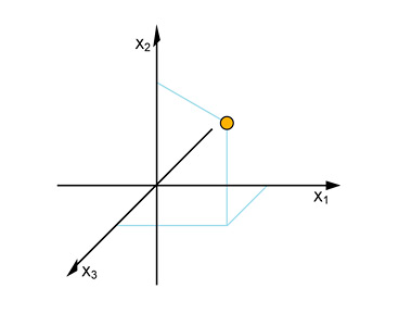
The essential idea is that one dimension of our data-table (the MSS) will become the Objects or points to be plotted. The other dimension of the table (the Versions) will become the new dimensions or coordinate axes of our Phase Space. To make this work, the numbers in any given column must be of the same kind and units, and it must be a simple scalar.
A Euclidean Metric
Something that is rarely talked about in simple introductions to PCA is the problem of the Metric of the Phase Space. The Metric of a 'Space' can be called a statement of the relations between points or coordinate axes, but more plainly, its about 'true distance' in space, regardless of direction.
If we are going to represent MSS (or anything else) as a set of points some fixed set of relative distances apart, then we have to be able to measure distances. We also need to be able to compare distances, independantly of direction or position.
And we need to be able to say things like "MS A is the same distance from MS B as MS F is from G", or "It is a greater distance than that between MSS P and Q." Only being able to reliably express these relations will allow us to group MSS together, and understand their true relation to other groups.
So distances in a space are expected to be constant (invariable) regardless of a change in orientation of coordinates. In fact, this property is mandatory if 'distance' in space is to have any objective meaning, and if a multi-dimensional model is to properly represent the 'distances' between objects.
In Euclidean Geometry, distances are expressed by the generalized Pythagorean Theorem. The theorem In algebraic terms, a2 + b2 = c2 where c is the hypotenuse while a and b are the legs of the triangle.
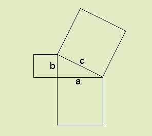
But the formula's most important use is in calculating the distance between any two arbitrary points, given their coordinates. The unknown distance is made the hypoteneuse, while the shorter sides correspond to the difference between the two points in X terms ( Δ x) and Y terms ( Δ y).
The equation is then solved for c:
( Δ x2 + Δ y2 )1/2 = c .
The distance formula is generalized for any number of dimensions:
distance = [ (Δ x1) 2 + (Δ x2) 2 + (Δ x3) 2...]1/2
For the formula to have any use, and for distance to be meaningful, it must be constant. But for this to be true, scales of the coordinate axes must be linear (the numbers must be equally spaced on the axis), and be of the same size units. Furthermore, the units must be the same as those used to measure distance in any direction in the space.
Said another way, we require our space to be a Euclidean Space, in which distance follows the generalized Pythagorean formula.
Why?
Because one of the first things we do in PCA is to take distance measurements of the objects in this space, to determine which axes efficiently cover the maximum variation in distance between the objects. Even though we do this indirectly (i.e., algebracially not graphically), its done using actual coordinates, and we rely upon calculations that use the generalized Pythagorean Theorem throughout the operation.
The PCA technique requires, and assumes, that the data columns to be operated on and converted into coordinate axes are linear in magnitude, are equivalent in nature and type, are expressed in the same units, and are capable forming an N-Dimensional Euclidean Space.
A PCA Transform and Projection Begins
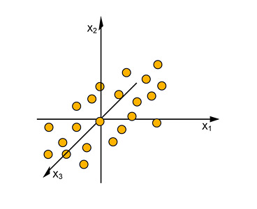
Obviously with a space having a large number of dimensions, we cannot visualize or recognise the patterns, or even make a useful model. The first part of the technique involves reducing the number of dimensions to something managable.
But if we just plot 3 columns of our data-table as a 3-Dimensional Space we may just get an arbitrary cloud of points in space with no apparent order or pattern, at least from the point of view our observed variables (the 3 selected columns).
Purpose and Goal of PCA
A model of the Observed Variables lets us down. No plain correlation or pattern seems to appear. These observed variables are called Manifest Variables to distinguish them from any Hidden Variables, that will expose patterns and possibly reveal underlying causes or processes.
The key with PCA is to find new hidden variables (in our current example, two) for the plot, that will organize the data and reveal underlying causes or effects. These hidden variables will become the new coordinate axes for a projection that reveals the hidden structure.
At the same time, the left-over hidden variables that retain unused information or complications that veil the pattern are ignored. This reduces the model back down to two dimensions, for a clean projection.
The unused information is treated like 'noise', and the isolated pattern is viewed as the 'signal'. In this way, PCA enthusiasts can talk of PCA as a "method of separating the signal from the noise", although strictly speaking this implies unsubstantiated assumptions about the data.
Step 1: Zeroing the Data - Subtract the 'mean'
For PCA to work properly, you have to subtract the mean (average value) from each of the data dimensions.
Subtracting the 'Mean'
The actual 'mean' that is subtracted from each entry is the average across each dimension. What is meant is actually simple: each 'dimension' is a column of data from the data-table.
We get the Mean Average by simply adding up all the entries, and dividing by the number of entries. This gives us the simplest and crudest kind of average value: the Mean. The formula is simple. If the set of entries for a column is:
X = [X1, X2, X3, ...Xn ]
...then the formula for the Mean average is:
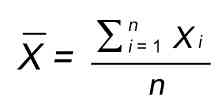
So, all the x values have x (the Mean of x) subtracted, and all the y values have y subtracted from them, etc. . This produces a data set whose mean (average value) is zero for every column (dimension).
What are we doing when we do this? This is something like finding the 'center of mass' for a floating cloud of particles. It places the Origin of our coordinate axes somewhere in the middle of the cloud.
By 'somewhere', we stress that this may not be the actual geometrical 'center'. We might think we want to do that when plotting a cloud, just as a photographer might center his 'shot' so that the subject is in the middle. This saves graph paper. But Zero Mean conversion is different.
The Origin is located at a 'center' that is really a weighted center, weighted by the number of points in each range of values, for each axis. So if there were for instance a lot of points in a certain range, this would 'pull' the Origin toward that group or cluster.
In order to plot all the points, (and save paper), we would then place the origin and the 'view-window' independantly:
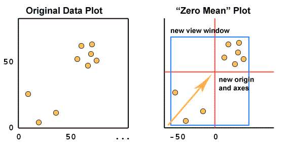
This is what the 'cross-hairs' and zero-lines in a PCA plot are all about. They show the weighted 'center' of the data, and its spread from this core in various directions. The reason that these lines are not centered themselves is that the viewport has to accomodate all the plotted points, and is chosen independantly.
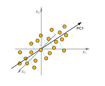
Step 2: The 1st Principal Component Axis
Calculating the Principal Component Axis is the first step in a multivariate projection. We draw this new co-ordinate axis along the line of maximum variation of the data. That is, in a way that spans the maximum length or spread of the cloud of points. It can also be called a "line of best fit".
This axis is known as the First Principal Component Axis (PC1 in the picture). All the observations are projected down onto this new axis and the score values are read off. These become the new entries for a new Hidden Variable, the First Principal Component. This variable becomes a column in a new 'transformed' data-table with all new columns and entries.
This First Principal Component is said to "explain" as best as possible, the spread of the "Observations" (MSS) in our original 3-dimensional space. This spread is expressed as a percentage of the total variation in position, and is said to "explain" that % of it.
From the picture below, you can see that this involves somehow minimizing the distances of all the points to this line. That could be a pretty messy job, involving a lot of measuring and adjustment: luckily there is a handy technique that does this for us automatically.
In Matrix Algebra we can calculate the Eigenvectors, which happen to be the very axis lines we are looking for. We will explain how to do that later. The important point is that these Eigenvectors are also a set of orthogonal (at right angles) lines in space. But this time they are aligned to our data, and can serve as an alternate set of axes.
(1) Euclidean Vector Space Needed
In this application of Matrix Algebra, the coordinate space is treated as a Vector Space, and the points in space are treated as Vectors. This Vector Space and the coordinate points in it must obey a strict set of Tranformation Rules, and the Vector Space must be Euclidean.
All of the distances between points in this Vector Space, for instance, the length of Eigenvectors, are calculated using the Generalized Pythagorean Formula:
For instance, if En is an Eigenvector, the Length of that vector is:
LE = [ X12 + X22... + Xn2 ] 1/2
Once again we see that the data must already be in a form that conforms to coordinates in a Euclidean Space, in order for proper distance calculations to be made.
(2) Square Data Table Needed
Now we run into one more snag! For large numbers of dimensions or observations, we have to resort to Eigenvector techniques. But Eigenvectors can only be found in square matrices. That is, our data table must have the same number of columns as it has rows.
If we have more columns than rows, or vice versa, we have to disgard some data, often a signficant amount! Or we have to break it down into smaller squares, and apply PCA techniques separately to the pieces, an obviously arbitrary and dubious method.
Once again, we are either artificially 'designing' the experiment to fit the method, biasing the result, or we are going to needlessly complicate the process of applying PCA, again with questionable results.
Even with a relatively large 'sample' of our data-table, the actual Eigenvector values may be way off from the actual 'maximum spread' axes.
Step 3: The Second Principal Component Axis
We now add a second principal component – PC2 in the picture. After PC1, this defines the next best direction for approximating the original data and is orthogonal (at right angles) to PC1.
To do this graphically, we would keep the PC2 line at a right angle to the PC1 line, and rotate it around until it was spanning the widest part of the cloud. In actuality, we simply select the 2nd largest Eigenvector, using the Eigenvalues as a guide.
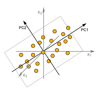
These two axes give the "best possible" two-dimensional window into our original 3-dimensional data, accounting for the largest % of the original variation.
Best View?
This opinion of 'best view' is based upon the idea that the projection will maximize the distance between the points in the projection. This is supposed to give maximum clarity and allow accurate identification of patterns or groups in the data.
This approach may be generally 'sound' as the best compromise for a projection, when nothing is known about the data other than the range of its values. But a little reflection should reveal that it is hardly an effective pattern-detecting method.
In fact, other than giving a very basic snap-shot of the data, the PCA technique is not very useful, except in cases where the data is already in a form or has features that are conveniently 'lucky' for this crude projection technique.
We'll see shortly how even a careful and correct application of PCA can catastrophically fail.
Because the success of the method is entirely dependant upon the data itself, it is a wholly unreliable and unrealistic technique for general data analysis.
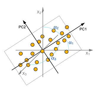
Where are the Original Variables?
The new axes PC1 and PC2 replace the original variables but we can still relate back to the old variables by measuring the angles between those axes and the Principal Component axes.
A small angle would mean that the variable has a large impact on the spread because it is almost aligned with a principal component. A large angle from any principal axis indicates less influence (the maximum angle possible is 90º ignoring sign reversals, but with N-dimensional spaces there are more possibilities, e.g., a given axis can be perpendicular to more than two other axes.).
For example, a variable lying at 90º to a principal component has no influence on that component whatsoever. So the influences of the old variables can be determined from the loading plot, provided the change of angle is clearly indicated.
Once the PC2 axis is fixed, the observations (MSS) will be projected down onto the plane made from these two axes to create the score plot. Imagine the shadow cast by a three-dimensional (or multi-dimensional) swarm of points onto a wall.
With the light source positioned optimally, the underlying structure of the data is hopefully revealed even though the dimensionality of the data has been dramatically reduced (and spacial information has been lost).
There is no doubt that the PCA method does do what it says it does: It efficiently displays the spread of the data-points according to the Covariance Matrix. What is that? Its a collected set of measurements that summarize the basic spread of all the variables.
That is, PCA, done properly will give us the projection that has the widest spread of the data points possible in two dimensions. It does this without adding any further distance distortion other than that caused by dropping the dimension perpendicular to the projection.
But is this 'data analysis'? No. There may be all kinds of critically important geometrical relationships in the data-points that will be left undiscovered. The PCA method has about as much chance of tripping over these as a farmer searching for a needle in a haystack without a magnet.
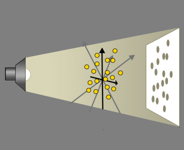
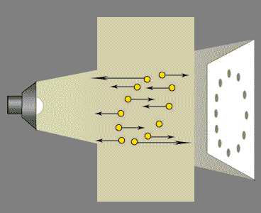
What the PCA Projection Missed...
To show the whopping errors possible with PCA, we need only imagine rotating the Principle Component Axis (the one "accounting" for the greatest % of the spread!) end over end as we continue the projection:
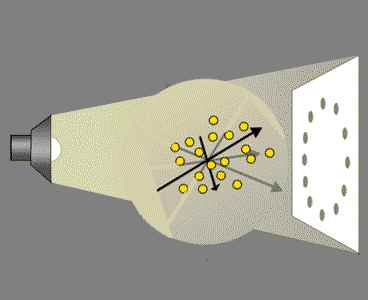
What happened? On a set of axes not related to either our original data Variables, or the PCA axes, there was a correlated sine/cosine function, a Hidden Variable.
By freely rotating our cloud under a light, we were able to reveal the hidden pattern, which in turn suggests a hidden and simple rule organizing and possibly 'causing' the readings.
A 'by the book' PCA analysis failed to expose the key pattern in the data, while a simple Rotation Transform, a rotation of the data through a series of angles, nailed it. At the same time, this exercise shows that PCA projections don't really expose hidden variables in data, and can't.
How did the PCA method fail?
Suppose the data plots were position recordings. The object is a tiny magnet suspended in an electromagnetic field. The motion of the object under investigation was a simple circular orbit. Unfortunately, the observer's apparatus is tilted at 45 degrees and mounted in a moving truck travelling along a bumpy road. This adds a random vertical component to each position of the object at 45 degrees to the orbit:
Now the spread of the position measurements is larger on a non-relevant axis than on the important pair, the plane of the orbit.
One might think this kind of situation is rare. But the opposite is the case. Raw field data is quite often compounded by multiple hidden factors influencing the recorded entries. It only takes a couple of layers of influencing factors to totally defeat a PCA projection.
The PCA technique actually failed because there was too much 'noise' in the data, that is, unimportant or unwanted measurements. But one of the claims of PCA proponents is that it is able to 'separate the noise from the signal'.
The sobering fact is that the noise must be an order of magnitude smaller than signal for PCA to work! But if that was the case above, PCA techniques would be redundant. The essential quality and pattern in the data (a circular orbit) would be obvious from almost any orientation or projection. We wouldn't need Principal Components at all.
This is true generally. If the data-table properly records the positions in a Euclidean space, clusters, patterns of all kinds will retain their essential shapes and groupings from many angles. If the 'noise' level is too high, PCA cannot reliably help.
What then is PCA?
And what is it really good for? PCA is a good method for displaying spacial relationships or affinities between observations, when the data is already in the right form, relatively free of error, and well-behaved. It is an excellent final polish, when an experiment has already been designed properly, and unwanted influences have been eliminated from consideration, and the key variables are already identified.
It is best when the data-points in the modeling Space DON'T have any special ordering, or pattern, other than an uneven spread (varying mean and median deviations) in the space. In this case, PCA does a good job as a general compromise for a 'best view' of the data, giving maximum separation.
In other words, it has no special value for pattern recognition, or separating 'signal' from 'noise'. This seems to be an accumulated popular mythology in part caused by its apparent success in various applications. But much of this seems to have more to do with experiment design and coincidental data patterns than with any inherent value in PCA itself.
PCA in Textual Criticism
A Real-World Example: Weiland Willker on the PA
Recently, W. Willker attempted to apply PCA to the problem of grouping MSS containing the Pericope de Adultera (John 7:53-8:11). In his 40 page 'Textual Commentary', Vol. 4b, The Pericope de Adultera (5th ed. 2007), Willker spends about 3 pages outlining his application of PCA.
Willker's work is deficient, because it lacks scientific rigor and focus, and uses outdated and inappropriate rhetorical methods . The essential flaws in Willker are these:
(1) Instead of presenting the full evidence in an unbiased manner, he slants the presentation to favour his own personal judgement. While typical of this field in the past, it is wholly unacceptable as 'science'. For instance,
a) Willker groups all the MSS which omit the passage together as though they were a homogenous group of equal authority, but fails to provide any dates for any of the witnesses. Yet when he lists the MSS which contain the passage, he breaks up the witnesses into subgroups and special cases, and lists the principal witnesses by century.
b) Willker is still listing 'Codex X' as though it were an ancient uncial MS omitting the passage. But actually this is a 13th century commentary which naturally skips over the passage during the public reading for Pentecost. Its not a gospel MS, its not an uncial, and its not an ancient manuscript at all. Even Wallace and friends on BIBLE.ORG had corrected this boner back in 1996. Its ten years later, and Willker has revised his pamphlet (5th ed.) four times as of Jan 2007, but still hasn't corrected these flaws.
c) Willker completely omits any discussion of the umlaut evidence and its significance in his PA article, even though this is critically important for evaluating codex B, and its witness concerning the PA.
(2) Willker makes several claims but fails to present key evidence. For instance,
a) he claims to have "made a reconstruction of [the missing pages of Codex A] from Robinson's Byzantine text with nomina sacra." - but never produces the pages, an easy task, allowing other scholars to evaluate his claim. The purpose of the measurement is to 'prove' that the missing pages could not have contained the pericope, yet no actual evidence is ever offered. (pg 6)
b) he claims to have done a PCA upon all the major MSS groups, but fails to provide the text he used for each group, the MSS he considers to be in each group, or any of the calculations used to create his data or chart. In fact, he doesn't provide an explanation or even an outline of his methodology. This is not a standard technique, but rather a novel one: his own personal application of his own personal method. A failure to provide the key documentation is wholly unacceptable in a scientific work making a scientific claims. (pg 18-21)
c) His discussion of the 'internal evidence' is limited to the examination of single words and short phrases, a practice recognized long ago as too subjective and fraught with error to be really useful. (pg 14).
In every other related field (for instance NT Aramaic studies) this practice was abandoned nearly 60 years ago. (see Casey, Aramaic Sources of Mark's Gospel, for a good review of the problems with 19th century 'stylometric' techniques. Speaking of Meyer (1896), Casey says, "The great advance which he made was to offer reconstructions of whole sentences" p.12. Criticising Torrey (1937), Casey says, "Torrey also deals often with only one or two words, which greatly facilitates playing tricks." p. 23. On Dodd (1935), Casey notes tellingly, "A single word is used to 'clear up' the problem...by using [only] one word, Dodd avoided the main questions." p. 27.)
The result is that in spite of some mitigating positive features, such as his brief discussion of Ehrman's evidence on Didymus, Willker's paper is not really a useful presentation of the evidence.
Willker's Application of Principal Components Analysis
Nonetheless, Willker's paper is one of the few that attempts to introduce PCA techniques to NT Textual Criticism. Here is the relevant section of Willker's paper on the Pericope de Adultera:
Textual groups [Willker, ibid pg 21-23]
Plummer (1893, in his commentary) notes 80 variants in 183 words (and there are probably many more), which makes the PA that portion of the NT with the most variants.
It is an interesting fact that the witnesses for the PA group different than in the rest of John. Also interestingly there is NO Byzantine text of the PA. Robinson (Preliminary Observations): "The same MSS which generally contain a Byzantine consensus text throughout the Gospels nevertheless divide significantly within the text of the PA." Robinson thinks that there are about 10 different "texttypes" of the PA. The version in Codex D is clearly not the parent of any of these, but it "must represent a near-final descendant of a complex line of transmission." Two minuscules, 1071 and 2722 have a very similar text as D in the PA (see below). The close relation of 1071 to D has been discovered by K. Lake, that of 2722 by M. Robinson. 1071 and 2722 are more closely related to each other than D/1071 or D/2722 in the PA (9 agreements against 2 and 3).
The following table is the result of a Principal Component Analysis (PCA) from Swanson's data (image see below):
| ... | Textual groups:[sic] | TCG name |
von Soden | # of dev. from txt | # of MSS |
| • | M, G, f1, 892, NA | f1-text | μ1 | 4-8 | >5 |
| • | S, W, 28 | S-text | μ2, μ3 | 8-9 | >60 |
| • | (E, G, H), K, 2, 579 | E-text | μ5, μ7 | 17-21 | μ5 280; μ7 260 |
| • | D, 1071, 2722 | D-text | μ1 | 13-14 | 3 |
| • | U, 700 | U-text | μ6 | 19 | 250 |
| • | L, f13, 1424mg | f13-text | μ4 | 17-20 | >30 |
[MSS] 892 and 1424mg have been added from NA/SQE [to the PCA analysis.]
. The first two groups are very similar, the last two are also clearly related. Basically there are four extreme groups:
1. the f1, S-text: (M, G, f1, 892), (S, W, 28)
2. the E-text: (E, F, G, H), K, P, 2, 579
3. the D-text: D, 1071, 2722
4. the U, f13-text: (U, 700), (L, f13, 1424mg)
The group that comes nearest to the reconstructed autograph (NA) is the f1-text. This is a remarkable, and almost unknown fact for f1. The S-text is also quite good.
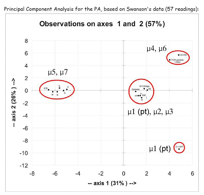
The other three groups are roughly equally far remote from the original text, but in different directions. Principal Component Analysis for the PA, based on Swanson's data (57 readings):
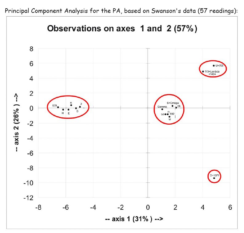
Please note that this image shows 2 dimensions only. Taking the third dimension into account one gets an additional, but smaller separation, e.g. (U, 700) is somewhat removed from (L, f13, 1424mg). I can differentiate the above mentioned 6 groups.
To check the correctness of the above result, I have carried out the same PCA analysis with the data from SQE. Even though the noted witnesses in NA are not completely the same, the result is the same, we get the same 4 major groups noted above. Von Soden's labels are not very fitting, e.g. he puts f1 into the same group as D, but they are very different. On the other hand he distinguishes μ2 and μ3, μ4 and μ6 and μ5 and μ7, which are very similar respectively. Strange.
Unfortunately I have no reliable information as to how many MSS support each group. The numbers above are from Hodges & Farstad's Majority Text edition, derived from von Soden. Acc. to von Soden the U-text μ6 and the E-text μ5 were the definitive types of the Byzantine era. But one cannot trust von Soden, his groupings are partly wrong and misleading.
With more data from more MSS, it is probably possible to make more precise statements regarding the f1- and S-texts. It might be that there are clearly distinguishable subgroups, the same is possible within the E-text. It is also possible that completely new groups show up."
(W. Willker, A Textual Commentary on the Greek Gospels, Vol. 4b,
The Pericope de Adultera: Jo 7:53 - 8:11 (Jesus and the Adulteress) 5th edition 2007)
Willker's Application of PCA: An Overview
Willker's Belief
"It is my belief that Multivariate Analysis in its many variants is THE TOOL for MSS grouping."
(from Willker's Introductory Article on PCA online at:
http://www1.uni-bremen.de/~wie/pub/Analysis-PCA.html)
It seems quite clear what Mr. Willker thinks about how to catalog and group MSS.
PCA (Principal Component Analysis) is only one family of a set of techniques that can be classified under the rubric "Multivariate Analysis", which as a general category of mathematical tools and techniques is pretty vague, although more than adequate to function as a sub-group of general statistical techniques and methods.
But by Willker's choice and application of PCA, it is pretty clear that this is what he basically has in mind.
Willker's Purpose
Again from the above quotation, and indeed his application of PCA throughout the section extending from page 21-23 in the latest incarnation of his 'Textual Commentary' (5th ed. 2007 online), Mr Willker clearly intends to use the technique as a method of sorting MSS and defining 'groups'.
Willker's Method
Willker begins by quoting Plummer (1893) concerning the number of variants in this section. The purpose of this is to somehow distinguish the PA from other parts of John.
However, the actual data does not support Willker's claim that this "make s the PA that portion of the NT with the most variants". Plummer's out-of-date collations (now all but unavailable to modern readers) are all but useless, because (a) Plummer was working at a time when most MSS had not been collated, or even properly catalogued. (b) Plummer's sample collations were not selected on a scientific basis. (c) Plummer's raw data cannot be reworked either, since he did not provide enough detail to correlate his observations with modern MSS names and classifications of text.
Willker then quotes Maurice Robinson (1997) who estimates there are about ten different 'text-types' or groups for MSS containing the PA.
The 'M1' Group:
Willker then notes that two MSS (1071 and 2722) have been noted by textual critics (Lake and Robinson respectively) as belonging to the same family or group as Codex D. Yet the differences between between these two MSS and D are far greater than their differences between each other. (1071 and 2722 agree 9 times against D! versus 2 and 3 times against each other with D).
This little aside about the Group (D, 1071, 2722) should give the reader serious pause. On the one hand, both Lake and Robinson are seasoned expert textual critics very familiar with the text and issues. Against the appearance of the statistics, both critics group these MSS together rather than place 1071 and 2722 in a separate group from D.
Will Willker's PCA technique solve or illuminate this dilemma? Wait and see.
'Swanson', or just the UBS text?
Next Willker claims to base his PCA analysis from "Swanson's data". However there is a serious problem with this claim before we even get out of the starting gate.
The PCA chart shows Willker has actually chosen a list of the principal MSS used by the editors of the UBS text (under the guidance of Cardinal Martini and Metzger).
Similarly, the list of 'Important Variants" at the back of Willker's article seems to be simply the list of the critical footnotes found in the UBS text (NA27), along with a few personal added notes.
Swanson

What exactly is 'Swanson'?
'Swanson' is actually a series of books, edited by Reuben Swanson, which prints the major variants of 45 manuscripts classed as the 'most important' by Metzger and his crowd of textual critics. These naturally include the early papyrii and the 4th century ecclesiastical MSS like Codex Vaticanus (B) and Codex Sinaiticus (Aleph).
While this would be a significant and useful tool for NT textual criticism, naturally it reflects the bias and vested interests of the Roman Catholic hierarchy promoting the text of Vaticanus (B). With a forward by Metzger, there is no doubt where the Swanson series falls in terms of ideological flavour.
The usefulness of Swanson is limited further by the fact that many of the 45 MSS chosen don't even include the Pericope De Adultera. What is really needed is a book like Swanson's that gives the readings of the important Byzantine MSS, which actually contain the passage under investigation.
If Willker has consulted Swanson at all, it is not apparent where or how, or why it would make any difference, since Willker seems to have simply chosen the variation units and MSS opted by the UBS commitee as important for translators.
Willker shows no knowledge of any of the other variation units or individual variants of texts. (There are between 35 and 40 variation units clearly identifiable, which can be found in the apparatus/footnotes of Hodges/Farstad, Robinson/Pierpont, and Pickering online.)
In any case, consulting Swanson's detailed collations has not caused Willker to make any changes in the 9 variation units he has chosen to copy from UBS.
Consulting the UBS introduction is instructive. They warn the reader that many significant variants simply do not appear in the apparatus or footnotes at all, because the committee viewed these variants as 'not suitable for translators'.
Thus the UBS editors were actively 'guiding' translators by limiting their choices of text to translate and ignoring important textual variants that would be useful for evaluating MSS evidence. This practice is obviously cross-purposes to providing textual evidence useful for textual critical reconstruction.
Now we find Willker has simply adopted the UBS text and variants for his experiment.
This is also an important question in regard to what MSS to consider. The UBS editors chose a very small subset of the extant MSS, allowing in many cases only a handful of MSS to represent groups containing 300 or more MSS. In most cases, MSS were chosen *without* a proper collation of the MSS within a group. Instead, the previous groupings (circa 1900-1912) were simply adopted, even though many errors in groupings and collations have been noted from past critics and collators.
Likewise, Willker has simply adopted the small group of MSS favoured by the UBS editors. Is this a representative sample of extant groups of MSS generally? Not really. One of the remarkable things about the methodology of the UBS editors was their admission that they applied Claremont Profile Methods to many MSS, in order to group them, but not for inclusion in the apparatus, but actually to EXCLUDE them. Thus hundreds of MSS were rejected by the UBS committee because they were 'too Byzantine' in their text-type according to profiling.
Willker starts with the 'six groups' identified by UBS, and correlates them to the 'seven groups' of von Soden, but only using the MSS chosen by UBS.
Then he presents his own 'findings' using his application of PCA to this small sample of MSS. The result is he finds only 'four groups' (see chart).
We have thus moved from Swanson's collations of thousands of MSS, to von Soden's 7 groups, to Metzger's 6 groups, to Willker's 4 groups.
Clearly, detailed information about the MSS are being eliminated, groupings of the MSS previously made by experts is being ignored, and finally, a new grouping based upon PCA is being offered in place of the work previously accomplished.
Willker's Result
Here we have duplicated Willker's chart, but added the corresponding names of the groups identified by von Soden to show what Willker's results give.
Willker's method cannot distinguish between the two main groups, M5 and M7. This is a catastrophic failure of Willker's application of PCA to the MSS. It could be the result of not enough MSS, or not enough variants, but in either case the failure is startling.
Among the 1350 some odd MSS which have the PA, some 300 MSS display the M5 text, and another 280 have the M7 text. As von Soden noted, these are not just two clearly defined and easily identifiable groups.
(1) each group is well represented by a large number of MSS.
(2) each group is clearly defined by a rigid profile using the Claremont Profile Method.
(3) each group is utterly stable, with the majority of MSS in each group keeping a 95% agreement in text to the group-text.
(4) each group is a DOMINANT text, these being the ONLY two text-types seriously competing for dominance throughout the Middle Ages.
(5) each group has a body of unique readings not found in other groups or significant MSS.
This is why every other textual critic who has examined these verses is in agreement that at least M5 and M7 are clearly identifiable and distinguishable groups, even when they differ on the existance or borders of other less plain groups in the MSS base.
Next, we note that Willker's PCA (WPCA) fails to distinguish M4 from M6, and blurs M1, M2, and M3. The only reason WPCA manages to separate out Codex D is its incredibly high number of peculiar abberant readings.
Thus we find that WPCA is no substitute for proper collation, careful evaluation of individual variation units and readings, and the tried and true criteria for grouping MSS into useful and realistic clusters.
By his own results, Willker's method is a failure, a very crude measure of the affinity between MSS and the clustering of groups. His results are unambiguous, but plainly at variance with known MSS groups and the criteria which define them.
As to the discrepancy between WPCA and that of over 100 years of textual critical analysis, Willker responds:
"To check the correctness of the above result, I have carried out the same PCA analysis with the data from SQE. Even though the noted witnesses in NA are not completely the same, the result is the same, we get the same 4 major groups noted above."
Yet Willker does not even show his results of the 'new test' he has allegedly carried out. There is no second chart or table of results for us to compare. We only have Willker's word for it.
But even if this were provided, how does performing the same technique on similar data confirm the conclusion or the result? It can't.
What WOULD have supported Willker's results and conclusions would be the application of an entirely different technique, with the same result, i.e., four groups instead of seven.
But even in that hypothetical case, no answer to the established and proven criteria for identifying and defining groups or text-types has been offered.
The criteria are pretty much self-evident, and while there will always be 'poorly defined' groupings in real cases of sloppy copying or mixture, this is not a fault of the standard criteria for groups but rather a proof of their value.
In response to his contradiction with von Soden's classifcations, Willker says this:
"Von Soden's labels are not very fitting, e.g. he puts f1 into the same group as D, but they are very different. On the other hand he distinguishes μ2 and μ3, μ4 and μ6 and μ5 and μ7, which are very similar respectively. Strange."
Willker finds von Soden's results 'strange', but apparently doesn't understand the detailed collations which led von Soden to distinguish these groups.
"Unfortunately I have no reliable information as to how many MSS support each group. The numbers above are from Hodges & Farstad's Majority Text edition, derived from von Soden. Acc. to von Soden the U-text μ6 and the E-text μ5 were the definitive types of the Byzantine era. But one cannot trust von Soden, his groupings are partly wrong and misleading."
We find then that Willker doesn't even rely upon von Soden, but is relying upon Hodges & Farstad's brief summary of von Soden's work in their introduction.
So Willker has never read von Soden (its a massive two Volume German treatise on the Greek text, with over 100 pages on the PA alone, and has never been translated into English.).
Yet Willker is free to dismiss von Soden's work and slag it (an admittedly popular pastime among English-speaking critics, see for instance Streeter's performances.) as untrustworthy, "partly wrong and misleading".
We have to ask, who is really doing the misleading?
The bottom line
Willker's technique here (WPCA) simply fails to identify the known groups of MSS, established upon independant and reasonable criteria by many other investigators.
Its not really von Soden that Willker has to contend with, but rather already known well-established and reasonable features expected and actually found, which distinguish MSS groups among the extant NT manuscripts.
I initially only complained about Willker's failure to provide his data and a clear explanation and justification for his method. But now that we have examined it in detail, it can be seen to be full of holes, both in its content and its methodology.
Further, the results are all but useless. Willker has not usefully sorted the NT MSS into groups according to their text-type. And his insistence that his method is "THE TOOL" is unconvincing.
Willker's attempt to introduce PCA to textual criticism has been almost hysterically defended by some parties. (cf. http://www.iidb.org/vbb/showthread.php?t=198138&page=5 as an example)
By contrast, Mr. Willker himself is far more honest and humble about his skills and his work:
Disclaimer:
"I am no expert in textual criticism and statistics. I am a chemist by profession and TC is a hobby only.
I just used available tools and played with the data.
This paper is meant as a stimulation for a serious student to explore this field further and deeper.
It is my belief that Multivariate Analysis in its many variants is THE TOOL for MSS grouping. "
(Willker, in his introductory paper on PCA here:
http://www1.uni-bremen.de/~wie/pub/Analysis-PCA.html)
Mr. Willker's self-defense is refreshing, in comparison to the rhetorical posturing of others.
Willker's Readings Base
Here is Wieland originally offering his analysis to the textcrit forum on Yahoo Groups (Dec. 2004) :
Willker Message #262 on TextualCritism List
"A wile [sic] ago I posted a PCA analysis of the evidence in the PA in John from Swanson's data (57 readings). I have uploaded the image again here: ..."
(message #262, http://groups.yahoo.com/group/textualcriticism/message/262)
This notice is again peculiar. Here Willker is affirming his use of Swanson.
Yet the data in the chart show he is using the UBS critical apparatus, with its limited number of MSS.
If Willker used Swanson, he did not use ALL of Swanson, namely all the collated MSS that Swanson documented. This is clear from the number of actual MSS plotted on his chart.
Again, he says he used "57 readings". From this it remains unclear whether he means 57 actual independant variation units, or simply 57 variants (you can divide that number in half if most of the variation units are binary in nature = 28 units, or if triple readings are being counted, less than 20 units).
The currently known count of significant variation units is about 35-40 at most.
Its another case where simple documentation could clear up just exactly how and what Willker was measuring.
It would have been trivial to simply post his 'Excel' spreadsheet file online.
Reverse-Engineering Willker
From the chart it is clear that Willker has posted a Score Plot.
We can see that Willker has put the 1st Principal Component along the X -axis, and the 2nd along the Y-axis.
Assuming he really did use an Excel spreadsheet and an add-on package to calculate this, he must have started with an N x N data-table of numbers.
Counting the number of MSS in the plot, he seems to have had at least 15 independant texts. (Some have been doubled up, like D+1071, S+Omega, and f13+Lambda+1424, a whole family of MSS treated as a unit).
Its unlikely that f13 for instance was entered as separate MSS. Instead Willker probably used a printed critical text of this family. For one thing, the only access to the actual detailed readings of the MSS in this family are available as footnotes to text (f13 can be found on my website).
This shows that the claim that Willker didn't use predefined Groups of MSS (like f13 ) as input is plainly false, going by the labels Willker himself has used.
As a MS base, Willker has only used 15 MSS and one family ( f13 ) containing about a half-dozen useful MSS that can witness the text.
That's right: Willker has used about 20-25 MSS for his PCA group analysis. The remaining question is, does Willker's 20 MS sample adequately represent the seven already identified texts distinguished by von Soden?
According to his own list, Willker believes he has represented all the groups, but some of his own sample groups are doing 'double-duty', representing two or more of von Soden's groups.
Remarkably, Willker uses only THREE MSS to represent two whole Groups: M3 and M2 are represented by only S, Omega, and MS 28.
Willker uses only SIX MSS to represent two more whole Groups, representing some 700 MSS.
It hardly seems surprising that Willker is unable to distinguish the Groups in either of these clusters of MSS.
One important question that comes up, since Willker has crapped all over von Soden as 'inaccurate' and 'unreliable', is what about more recent collations and investigations into the groupings of these MSS?
Willker himself notes that Maurice Robinson, probably the world's leading living expert on this passage at this time, "thinks that there are [actually] about 10 different text-types of the PA. The version in Codex D is clearly not the parent of any of these, but it "must represent a near-final descendant of a complex line of transmission."
Robinson is the only man alive to have personally collated ALL the 1,350 extant continuous-text MSS that contain the passage, as well as a 1,000 Lectionaries.
So the tendency of recent scholarship is to find MORE text-types (Groups) within the available MS tradition, not less.
Yet Willker's plot, based on only a handful of MSS, shows only 4 groups.
This also means that in order to do a PCA plot, Willker must have had at least 15 columns, but no more than 25 columns, of Variation Units. But we know that all the critical texts of the PA show between 30 and 40 Variation Units.
If Willker really did a PCA plot, then he must have ignored a significant number of the variation units, as well as the vast bulk of MSS.
Such a procedure can only be described as poking out one eye, in order to see the lay of the land better.
Can this really be a better way to tease out the delicate groupings of 1,350 MSS falling into apparently at least 10 different text-types?
No. What Willker has actually done, is to roughly 'group' the manuscripts he has sampled, on the basis of a small subset of readings and variation units. He himself hints that this is not a real categorization or final detailed picture of the groups:
"With more data from more MSS, it is probably possible to make more precise statements regarding the f1- and S-texts. It might be that there are clearly distinguishable subgroups, the same is possible within the E-text. It is also possible that completely new groups show up." (pg 23)
The second important question is posed when we naturally ask:
What Variation Units were used to characterize the MSS?
We would at least know this, if Willker had published his accompanying LOADING PLOT, which is necessary in order to interpret the SCORE PLOT.
This would assume that the Loading Plot was properly labelled, and told us by a name or I.D. number which Variant was being collated in each column.
The names would in turn refer to a list of Variation Units, like the ones in his own appendix.
Note that in Willker's Appendix, he only lists 13 Variation Units of note.
But to have done a PCA plot he would have required a minimum of 15 Units. The Data Table has to be Square, having the same columns as rows, in order to use PCA software that calculates Eigenvectors and Eigenvalues.
Why the discrepancy? Willker must have used a different number of Units, or divided them up differently in his PCA Data-Table.
One way to hide these problems, and avoid other investigators challenging his findings, is to fail to produce the LOADING PLOT.
The Loading Plot would inevitably show an equal number of Variables, and be expected to be supported by a mapping and an explanation of the group clusterings found in the Score Plot.
Far from Willker's conclusion that there are (only) four groups of MSS, we rather conclude that an inadequate PCA technique was performed.
It looks like Willker cut corners with MSS, readings, supporting documentation, and proper analysis.
The reason is, Willker seems to have simply used the variants and MSS found in the UBS text produced by Metzger and Jesuit cardinal Carlo Maria Martini, the Roman Catholic Archbishop of Milan. Since 1967, the Cardinal has been one of the editors of the UBS Greek NT for 'translators'.
But no adequate PCA analysis can be performed on such a half-assed sampling of variants and MSS as presented in that 'student's text' of the NT.
Willker seems to have used PCA projection as simply a quick and dirty means of displaying the 'groups', without completing the necessary work of collating the MSS, or encompassing the full set of variants.
Naturally no rationale for the groupings is offered. No analysis was done.
The result is more predictable than the Score Plot.
We have been given a fuzzy amateur 'snapshot' of SOME of the MSS and SOME of the readings.
This would be like shooting from a bad angle, in the dark, while the camera was shaking, and the exposure and focus was maladjusted. And that's exactly what we get, an incomplete, inaccurate, and misleading picture of the groupings of the MSS.